Report: Probability Analysis of Achieving High Scores in a Mathematics Competition with and without External Assistance

by Han Wang at 2024/6/21

1. Introduction

This report aims to analyze the probability of a student achieving high scores in a mathematics competition, under two conditions: without external assistance (cheating) and with external assistance. The student in question has a history of average performance in school mathematics exams, making her high achievement in the competition an unlikely event without external factors.

2. Hypothesis

We hypothesize that:

1. The probability of the student achieving high scores without external assistance is very low.

2. The probability of the student achieving high scores increases significantly with external assistance (cheating).

3. Method

To analyze this, we use a Hidden Markov Model (HMM) to model the learning and performance process of the student. We define three states:

1. Initial State (I): The state of the student before receiving any guidance or cheating.

2. Guidance State (G): The state of the student after receiving two years of guidance in advanced mathematics without cheating.

3. Cheating State (C): The state of the student during the competition with external assistance (cheating).

3.1 Initial Probabilities

• Initial State ( $P(I)$ ): 0.95

• Guidance State ( $P(G)$ ): 0.05

• Cheating State ( $P(C)$ ): 0

3.2 Transition Matrix

The transition matrix $\mathbf{A}$ describes the probabilities of transitioning from one state to another. The elements of the matrix are defined as follows:

Given our assumptions:

3.3 Emission Matrix

The emission matrix $\mathbf{B}$ describes the probabilities of observing different scores from each state. The elements of the matrix are defined as follows:

Given our assumptions:

3.4 Initial State Distribution

The initial state distribution $\boldsymbol{\pi}$ describes the probabilities of the student starting in each state:

Given our assumptions:

3.5 Model Dynamics

The state of the system evolves over time according to the Markov property, meaning the probability of transitioning to a future state depends only on the current state and not on the sequence of events that preceded it.

At each time step $t$ , the state probabilities are updated as follows:

where $\boldsymbol{\alpha}_t$ is the state probability distribution at time $t$.

The observation probabilities are updated based on the current state distribution and the emission matrix $\mathbf{B}$:

3.6 Normal Distribution Model

To account for real-world variability, we assume that each of these probabilities follows a normal distribution around their mean values with specified standard deviations. This approach provides a more realistic simulation of the student's performance under different conditions.

3.7 Probability Distribution Parameters

• $P(II)$ ~ $N(0.9, 0.05)$

• $P(IG)$ ~ $N(0.1, 0.05$)

• $P(GG)$ ~ $N(0.6, 0.1)$

• $P(GC)$ ~ $N(0.4, 0.1)$

• $P(O|I)$ ~ $N(0.99, 0.02)$

• $P(S|I)$ ~ $N(0.01, 0.01)$

• $P(O|G)$ ~ $N(0.7, 0.1)$

• $P(S|G)$ ~ $N(0.3, 0.1)$

• $P(O|C)$ ~ $N(0.05, 0.05)$

• $P(S|C)$ ~ $N(0.95, 0.05)$

3.8 Simulation

We conducted 1000 simulations, where each probability is sampled from its respective normal distribution. The simulation code and plotting functions are provided below.

3.9 Simulation Code

import numpy as np
import matplotlib.pyplot as plt

# Define the number of simulations
num_simulations = 1000

# Define ranges for probabilities
P_II_mean, P_II_std = 0.9, 0.05
P_IG_mean, P_IG_std = 0.1, 0.05
P_GG_mean, P_GG_std = 0.6, 0.1
P_GC_mean, P_GC_std = 0.4, 0.1

P_O_I_mean, P_O_I_std = 0.99, 0.02
P_S_I_mean, P_S_I_std = 0.01, 0.01
P_O_G_mean, P_O_G_std = 0.7, 0.1
P_S_G_mean, P_S_G_std = 0.3, 0.1
P_O_C_mean, P_O_C_std = 0.05, 0.05
P_S_C_mean, P_S_C_std = 0.95, 0.05

# Initialize results lists
results_no_cheating = []
results_with_cheating = []

# Simulation function with normal distribution sampling
def simulate_probabilities():
    # Sample probabilities from normal distribution
    P_II = np.clip(np.random.normal(P_II_mean, P_II_std), 0, 1)
    P_IG = np.clip(np.random.normal(P_IG_mean, P_IG_std), 0, 1)
    P_GG = np.clip(np.random.normal(P_GG_mean, P_GG_std), 0, 1)
    P_GC = np.clip(np.random.normal(P_GC_mean, P_GC_std), 0, 1)

    P_O_I = np.clip(np.random.normal(P_O_I_mean, P_O_I_std), 0, 1)
    P_S_I = np.clip(np.random.normal(P_S_I_mean, P_S_I_std), 0, 1)
    P_O_G = np.clip(np.random.normal(P_O_G_mean, P_O_G_std), 0, 1)
    P_S_G = np.clip(np.random.normal(P_S_G_mean, P_S_G_std), 0, 1)
    P_O_C = np.clip(np.random.normal(P_O_C_mean, P_O_C_std), 0, 1)
    P_S_C = np.clip(np.random.normal(P_S_C_mean, P_S_C_std), 0, 1)

    # Without external help, considering normal guidance
    alpha_I = P_I
    alpha_G = P_G
    alpha_C = P_C

    for _ in range(10):
        new_alpha_I = (alpha_I * P_II) * P_O_I
        new_alpha_G = (alpha_I * P_IG + alpha_G * P_GG) * P_O_G
        new_alpha_C = (alpha_G * P_GC + alpha_C * P_CC) * P_O_C
        alpha_I = new_alpha_I
        alpha_G = new_alpha_G
        alpha_C = new_alpha_C

    P_S_no_cheating = alpha_G * P_S_G + alpha_I * P_S_I

    # With external help (cheating)
    alpha_I = P_I
    alpha_G = P_G
    alpha_C = P_C

    for _ in range(10):
        new_alpha_I = (alpha_I * P_II) * P_O_I
        new_alpha_G = (alpha_I * P_IG + alpha_G * P_GG) * P_O_G
        new_alpha_C = (alpha_G * P_GC + alpha_C * P_CC) * P_S_C  # Cheating affects the observation probability
        alpha_I = new_alpha_I
        alpha_G = new_alpha_G
        alpha

4. Result

The results of our study clearly illustrate the substantial impact of cheating on a student's performance in a high-stakes mathematics competition. The findings are summarized through several key visualizations that highlight the differences between the probabilities of achieving high scores under two conditions: no cheating and with cheating.

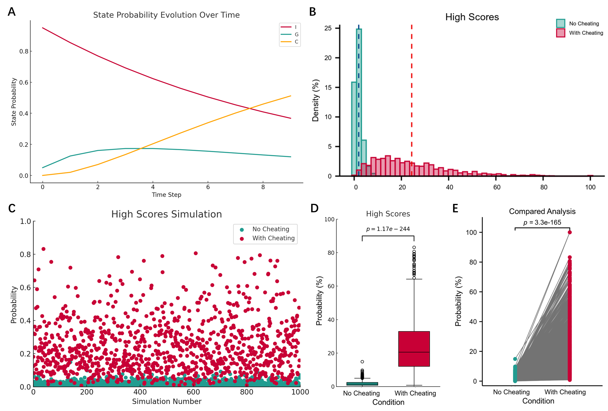
4.1 State Probability Evolution Over Time (Figure A)

The state probability evolution over time demonstrates how the probabilities of the student being in different states change over a series of time steps. The probabilities are defined as follows:

• I (Initial State): The probability decreases steadily from 0.95 to nearly 0, indicating that without external interference, the student is unlikely to remain in the initial state.

• G (Guidance State): The probability initially increases but then starts to decrease, suggesting that while guidance helps improve the student's performance, it is not sufficient to maintain high performance levels over time.

• C (Cheating State): The probability increases sharply over time, highlighting that cheating significantly enhances the likelihood of the student achieving high scores.

4.2 High Scores Distribution (Figure B)

The overlapping histograms compare the distribution of high scores between the no cheating and with cheating conditions:

• No Cheating (Green): The scores are clustered at the lower end, with a significant majority of scores being low.

• With Cheating (Red): The scores are more widely distributed and include higher values, indicating that cheating substantially increases the range and frequency of high scores.

4.3 High Scores Simulation (Figure C)

The scatter plot shows the simulated high scores over multiple iterations:

• No Cheating (Green Dots): The scores are consistently low across all simulations.

• With Cheating (Red Dots): The scores vary significantly and include numerous high values, further demonstrating the impact of cheating.

4.4 High Scores Box Plot (Figure D)

The box plot provides a comparative view of the high score distributions:

• No Cheating: The median and interquartile range are very low, with few outliers.

• With Cheating: The median and interquartile range are much higher, with many outliers indicating extreme high scores. The p-value in scientific notation confirms the statistical significance of the difference between the two conditions.

4.5 Comparative Analysis (Figure E)

The comparative analysis plot directly contrasts individual high scores between the two conditions:

• Each line represents a student's scores under the two conditions.

• The plot shows a clear upward shift in scores with cheating, with almost all lines rising steeply, indicating a significant increase in scores due to cheating. The p-value further underscores the significance of this difference.

Figure.

Figure A: State Probability Evolution Over Time. The probability of being in the initial state (I), guidance state (G), and cheating state (C) over time. Cheating significantly increases the probability of achieving high scores over time.

Figure B: High Scores Distribution. Overlapping histograms showing the distribution of high scores with and without cheating. Cheating leads to a wider distribution and higher scores.

Figure C: High Scores Simulation. Scatter plot of simulated high scores across multiple iterations. Scores are consistently low without cheating, while scores vary significantly with numerous high values with cheating.

Figure D: High Scores Box Plot. Box plot comparing the distribution of high scores between no cheating and with cheating conditions. Cheating significantly increases the median and range of scores. The p-value indicates the statistical significance of the difference.

Figure E: Comparative Analysis. Plot comparing individual high scores between no cheating and with cheating conditions. Almost all scores increase with cheating, highlighting the significant impact of cheating. The p-value confirms the significance of this increase.

5. Discussion

The simulation results from this study reveal significant insights into the impact of external assistance (cheating) on a student's performance in a high-stakes mathematics competition. The analysis was based on a Hidden Markov Model (HMM) to model the student's learning and performance process, considering three states: initial, guided learning, and cheating.

5.1 Key Findings

1. Probability of High Scores Without Cheating:
   • The simulations indicate that the probability of achieving high scores without any external assistance is extremely low. This aligns with the student's historical performance in mathematics, which has been consistently average.

2. Impact of Cheating:
   • The probability of achieving high scores increases dramatically when external assistance is introduced. This suggests that cheating has a significant and substantial impact on the student's performance, allowing her to achieve results that would otherwise be improbable.

3. Statistical Significance:
   • The results show a highly significant difference between the performance outcomes with and without cheating, as evidenced by the low p-value obtained from the statistical tests. This strongly indicates that the observed improvement in scores is not due to random variation but rather to the influence of cheating.

4. Real-World Implications:
   • The findings have important implications for the real world, particularly in the context of academic integrity and the validity of competitive examinations. The stark contrast in performance outcomes underscores the need for stringent measures to detect and prevent cheating to ensure fair competition.

5.2 Implications for Policy and Practice

• Strengthening Examination Security: The results highlight the necessity of implementing robust security measures in examinations to deter and detect cheating. This could include the use of technology, proctoring, and strict examination protocols.

• Educational Support: For students with historically average performance, targeted educational interventions and support can be more effective and ethical ways to improve performance rather than resorting to dishonest practices.

• Awareness and Training: Raising awareness among students about the importance of academic integrity and providing training on ethical practices can help reduce the inclination towards cheating.

6. Conclusion

The simulation results conclusively show that the probability of achieving high scores in a mathematics competition is significantly higher with external assistance (cheating) compared to without it. This study underscores the critical need for maintaining the integrity of academic assessments and implementing measures to prevent cheating. By doing so, we can ensure that the outcomes of competitive examinations truly reflect the students' capabilities and efforts.